<?xml version="1.0" encoding="utf-8"?><feed xmlns="http://www.w3.org/2005/Atom" xml:lang="en"><generator uri="https://jekyllrb.com/" version="4.4.1">Jekyll</generator><link href="https://pmantini.github.io/profile/feed.xml" rel="self" type="application/atom+xml"/><link href="https://pmantini.github.io/profile/" rel="alternate" type="text/html" hreflang="en"/><updated>2026-04-05T19:03:37+00:00</updated><id>https://pmantini.github.io/profile/feed.xml</id><title type="html">Pranav Mantini</title><subtitle>Senior Researcher and Lecturer at the University of Houston. Specializing in Computer Vision and Machine Learning. </subtitle><entry><title type="html">Multi-Modal Spaces</title><link href="https://pmantini.github.io/profile/blog/2026/clip/" rel="alternate" type="text/html" title="Multi-Modal Spaces"/><published>2026-04-03T14:24:00+00:00</published><updated>2026-04-03T14:24:00+00:00</updated><id>https://pmantini.github.io/profile/blog/2026/clip</id><content type="html" xml:base="https://pmantini.github.io/profile/blog/2026/clip/"><![CDATA[<ul id="markdown-toc"> <li><a href="#a-simple-view-of-cnns-or-transformers" id="markdown-toc-a-simple-view-of-cnns-or-transformers">A Simple View of CNNs or Transformers</a> <ul> <li><a href="#vision-models" id="markdown-toc-vision-models">Vision Models</a> <ul> <li><a href="#embedding-spaces-for-retrieval" id="markdown-toc-embedding-spaces-for-retrieval">Embedding Spaces for Retrieval</a> <ul> <li><a href="#example-image-based-search" id="markdown-toc-example-image-based-search">Example: Image-Based Search</a></li> </ul> </li> </ul> </li> <li><a href="#textual-models" id="markdown-toc-textual-models">Textual Models</a></li> </ul> </li> <li><a href="#mult-modal-spaces" id="markdown-toc-mult-modal-spaces">Mult-Modal Spaces</a> <ul> <li><a href="#the-cross-modal-search-problem" id="markdown-toc-the-cross-modal-search-problem">The Cross-Modal Search Problem</a></li> <li><a href="#multimodal-spaces" id="markdown-toc-multimodal-spaces">Multimodal spaces</a> <ul> <li><a href="#challenges-to-achieving-harmony" id="markdown-toc-challenges-to-achieving-harmony">Challenges to Achieving Harmony</a></li> </ul> </li> </ul> </li> <li><a href="#clip-contrastive-language-image-pre-training" id="markdown-toc-clip-contrastive-language-image-pre-training">CLIP (Contrastive Language-Image Pre-training)</a></li> </ul> <p>Every modern AI model, whether it processes images or text, lives in a world of <strong>Embeddings</strong>.</p> <h3 id="a-simple-view-of-cnns-or-transformers">A Simple View of CNNs or Transformers</h3> <h4 id="vision-models">Vision Models</h4> <p>If you consider a Convolutional Neural Network (CNN) or a Vision Transformer that are commonly used for image classification, you can conceptually split it into two distinct functional units:</p> <ul> <li> <p><strong>The Feature Extractor (The Encoder):</strong> Consider images of dogs: they come in different breeds, sizes, and colors. They can be photographed from different angles, in different lighting, or even obscured by noise and clutter. However, they all relate to a specific concept “dog” despite having large variance in pixels and their orgnizations.</p> <p>The goal of a robust Encoder is to ignore these superficial variations and focus on the semantic content. It must map a blurry or a top-down photo of a Golden Retriever, or a high-resolution side profile of a Husky to high-dimensional vectors. Such that these vectors when views in a geometric space (embedding space) they cluster together into groups represnting semantic concepts. The encoder in essence is performing a mathematical “distillation” process to cast semantically equalent concepts into clusters.</p> <p>In the chart below, see how the “Dogs” cluster stays together despite being “Noisy” (spread out), while the “Vehicles” cluster remains distinct. This demonstrates how the encoder handles variance while maintaining semantic grouping:</p> </li> </ul> <pre><code class="language-plotly">{
  "data": [
    {
      "x": [1.1, 1.5, 0.8, 1.2, 1.4, 0.9, 1.3, 1.1],
      "y": [5.1, 5.5, 4.9, 5.2, 5.6, 4.8, 5.3, 5.0],
      "mode": "markers",
      "type": "scatter",
      "name": "Images of Dogs",
      "marker": { "color": "rgb(200, 16, 46)", "size": 10 }
    },
    {
      "x": [4.1, 4.5, 3.8, 4.2, 4.4, 3.9, 4.3, 4.1],
      "y": [1.1, 1.5, 0.9, 1.2, 1.6, 0.8, 1.3, 1.0],
      "mode": "markers",
      "type": "scatter",
      "name": "Images of Vehicles",
      "marker": { "color": "rgb(0, 123, 255)", "size": 10 }
    }
  ],
  "layout": {
    "title": "Robust Semantic Clustering in 2D",
    "xaxis": { "title": "Feature Dimension 1", "range": [0, 6] },
    "yaxis": { "title": "Feature Dimension 2", "range": [0, 7] },
    "shapes": [
      {
        "type": "circle",
        "xref": "x", "yref": "y",
        "x0": 0.6, "y0": 4.5, "x1": 1.7, "y1": 5.8,
        "line": { "color": "rgb(200, 16, 46)", "dash": "dash" },
        "opacity": 0.3
      },
      {
        "type": "circle",
        "xref": "x", "yref": "y",
        "x0": 3.6, "y0": 0.6, "x1": 4.7, "y1": 1.8,
        "line": { "color": "rgb(0, 123, 255)", "dash": "dash" },
        "opacity": 0.3
      }
    ],
    "annotations": [
      {
        "x": 1.1, "y": 6.2, "text": "Canine Neighborhood", "showarrow": false, "font": { "color": "rgb(200, 16, 46)" }
      },
      {
        "x": 4.1, "y": 2.1, "text": "Vehicle Neighborhood", "showarrow": false, "font": { "color": "rgb(0, 123, 255)" }
      }
    ]
  }
}
</code></pre> <ul> <li> <p><strong>The Classifier (The Head):</strong> The Classifier is the “Decision Maker.” It takes the high-dimensional embedding and computes the probability that it belongs to a particular class (e.g., Dog vs. Car).</p> <p>However, there is a fundamental rule in machine learning: The Classifier can only be as good as the robustness of the embedding features. If the Encoder is weak, the “Canine” and “Vehicle” embeddings will overlap in a messy, inseparable cloud. No matter how complex your Classifier is, it will struggle to draw a boundary between them. But if the Encoder is robust, it creates “Semantic clusters” that are distinct and can allow for good accuracy.</p> </li> </ul> <h5 id="embedding-spaces-for-retrieval">Embedding Spaces for Retrieval</h5> <p>Once we have a robust Embedding Space, we can do more than just classify images. We can use the geometry of the space for Matching and Retrieval.</p> <p>In a retrieval system, we don’t ask the model “What objects is in this image?” Instead, we ask, “what other images contain this object”. In order to achive this, we take a “Query Image,” find its coordinate, and look for its “Nearest Neighbors” in the database. This allows us to find visually and semantically similar items even if they don’t have a label.</p> <h6 id="example-image-based-search">Example: Image-Based Search</h6> <p>Imagine you are building a search engine for images in a database. A user uploads a query photo of a German Shepherd they saw on the street.</p> <ul> <li> <p>The Extraction: Your Encoder processes the photo and generates a unique embedding vector—a specific coordinate in your “Canine” neighborhood.</p> </li> <li> <p>The Search: The system calculates the mathematical distance (often using Cosine Similarity) between the query’s coordinate and every other image embedding in your database.</p> </li> <li> <p>The Result: The images with the “closest” coordinates are returned. Because your space is semantically robust, the top results won’t just be vehicles or any dogs; they will be German Shepherds with similar frame geometries, even if those specific attributes were never manually tagged by a human.</p> </li> </ul> <pre><code class="language-plotly">{
  "data": [
    {
      "x": [1.5, 1.6, 1.4, 4.0],
      "y": [5.2, 5.3, 5.1, 1.5],
      "mode": "markers+text",
      "type": "scatter",
      "name": "Database Images",
      "text": ["GS Alpha", "GS Beta", "GS Gamma", "Truck"],
      "textposition": "bottom center",
      "marker": { "color": "rgba(0, 0, 0, 0.3)", "size": 10 }
    },
    {
      "x": [1.55],
      "y": [5.25],
      "mode": "markers+text",
      "type": "scatter",
      "name": "Query: German Shepherd",
      "text": ["User Query"],
      "textposition": "top center",
      "marker": { "color": "rgb(200, 16, 46)", "size": 14}
    }
  ],
  "layout": {
    "title": "Retrieval: Finding a German Shepherd",
    "xaxis": { "title": "Feature Dimension 1", "range": [0, 5] },
    "yaxis": { "title": "Feature Dimension 2", "range": [0, 7] },
    "shapes": [
      {
        "type": "circle",
        "xref": "x", "yref": "y",
        "x0": 1.1, "y0": 4.7, "x1": 1.9, "y1": 5.8,
        "line": { "color": "rgb(200, 16, 46)", "dash": "dot" },
        "label": { "text": "Canine Neighborhood", "font": { "size": 10 } }
      }
    ]
  }
}
</code></pre> <h4 id="textual-models">Textual Models</h4> <p>While Vision models were learning to group pixels, Natural Language Processing (NLP) was undergoing a similar revolution. Instead of looking at pixels, models like BERT or GPT-style Transformers look at textual corpus to understand relationships between words, sentences, and contexts.</p> <p>The goal remains the same: to learn an embedding space where semantically similar words/sentences are grouped together. For example,</p> <ul> <li>The embeddings correspoding to “Dog” and “Puppy” should be close to each other compared to a non-related concept such as a Truck. (or)</li> <li>“Canine” and “German Shepherd” should fall into the same “neighborhood,” even if they don’t share a single letter in common.</li> </ul> <p>This allows for Semantic Search. If you search a database for the word “canine,” a robust text space knows to retrieve documents containing “dog,” because the model has learned that these concepts live in the same geometric region of the embedding map.</p> <pre><code class="language-plotly">{
  "data": [
    {
      "x": [4.2, 4.4, 4.0, 1.2],
      "y": [1.2, 1.5, 0.9, 5.2],
      "mode": "markers+text",
      "type": "scatter",
      "name": "Text Embeddings",
      "text": ["Dog", "Puppy", "Canine", "Truck"],
      "textposition": "top center",
      "marker": { "color": "rgb(128, 0, 128)", "size": 12, "symbol": "star"  }
    }
  ],
  "layout": {
    "title": "The Semantic Text Space (Unaligned)",
    "xaxis": { "title": "Language Dimension 1", "range": [0, 5] },
    "yaxis": { "title": "Language Dimension 2", "range": [0, 7] },
    "shapes": [
      {
        "type": "circle",
        "xref": "x", "yref": "y",
        "x0": 3.7, "y0": 0.6, "x1": 4.7, "y1": 1.8,
        "line": { "color": "rgb(128, 0, 128)", "dash": "dot" }
      }
    ],
    "annotations": [
      {
        "x": 4.2, "y": 2.2, "text": "Linguistic 'Canine' Cluster", "showarrow": false, "font": { "color": "rgb(128, 0, 128)" }
      }
    ]
  }
}
</code></pre> <h3 id="mult-modal-spaces">Mult-Modal Spaces</h3> <p>At this point, we have built two incredibly powerful geometric spaces: a Visual Space where images are orgnaized based on semantic content and a Textual Space where words/sentences with same semantic meaning are grouped together.</p> <h5 id="the-cross-modal-search-problem">The Cross-Modal Search Problem</h5> <p>We already know how to use these spaces individually:</p> <ul> <li> <p>We can use an image of a dog to search for other images of dogs in the Visual embedding space (Image-to-Image).</p> </li> <li> <p>Similarly, we can use keywords to search for related documents or sentences in the Textual space (Text-to-Text).</p> </li> </ul> <blockquote> <p>🔍What if we want to search for all images of a dog by specifying a keyword such as <strong>“German Shepherd”</strong>?</p> </blockquote> <h4 id="multimodal-spaces">Multimodal spaces</h4> <p>To solve the cross-modal search problem, We will need a joint space where image and text embedding can live in harmony. This is a unified geometric space where an image of a German Shepherd and the text string “German Shepherd” are mapped to the same (or very similar) coordinates.</p> <pre><code class="language-plotly">{
  "data": [
    {
      "x": [1.2, 1.4, 0.9],
      "y": [5.2, 5.5, 4.9],
      "mode": "markers",
      "type": "scatter",
      "name": "Image Embeddings (Dogs)",
      "marker": { "color": "rgb(200, 16, 46)", "size": 12, "symbol": "circle" }
    },
    {
      "x": [1.25, 1.45, 0.85],
      "y": [5.15, 5.45, 4.85],
      "mode": "markers",
      "type": "scatter",
      "name": "Text Embeddings (Dogs)",
      "marker": { "color": "rgb(128, 0, 128)", "size": 14, "symbol": "star" }
    },
    {
      "x": [4.2, 4.4, 4.0],
      "y": [1.2, 1.5, 0.9],
      "mode": "markers",
      "type": "scatter",
      "name": "Image Embeddings (Vehicles)",
      "marker": { "color": "rgb(0, 123, 255)", "size": 12, "symbol": "circle" }
    },
    {
      "x": [4.25, 4.45, 4.05],
      "y": [1.15, 1.45, 0.85],
      "mode": "markers",
      "type": "scatter",
      "name": "Text Embeddings (Vehicles)",
      "marker": { "color": "rgb(0, 128, 128)", "size": 14, "symbol": "star" }
    }
  ],
  "layout": {
    "title": "A Harmonious Multimodal Space",
    "xaxis": { "title": "Unified Dimension 1", "range": [0, 6] },
    "yaxis": { "title": "Unified Dimension 2", "range": [0, 7] },
    "legend": { "orientation": "h", "y": -0.2 }
  }
}
</code></pre> <h6 id="challenges-to-achieving-harmony">Challenges to Achieving Harmony</h6> <ul> <li><strong>The Dimensionality Mismatch</strong>: Vision and text models are often trained independently using different architectures. This means their “outputs” (the embedding vectors) rarely share the same shape. <ul> <li>A ResNet or Vision Transformer might produce a 512-dimensional vector.</li> <li>A BERT or GPT-based text encoder might produce a 768 or 1024-dimensional vector. Mathematically, you cannot compare a 512D point to a 768D point. They don’t even exist in the same space.</li> </ul> </li> <li><strong>The Semantic Disconnect</strong>: Even if we force both models to output the same number of dimensions, there is no reason for independently trained models to align. <ul> <li>The Vision model might learn that top-left space correspond to dogs.</li> <li>The Text model might learn bottom-right space correspond to dogs.</li> </ul> <p>Without a shared training objective, an image of a German Shepherd and the word “German Shepherd” will be scattered in completely different parts of their respective maps.</p> </li> <li><strong>Scaling &amp; Generalization</strong>: Even if we solve the dimensionality and alignment issues, training on small, curated datasets (like ImageNet) often fails to produce a truly “generalized” embedding space. To learn a space where any text can map to any image, we need hundreds of millions of diverse image-text pairs. Furthermore, Aligning these “Web-Scale” datasets requires massive computational resources to process the billions of contrastive relationships during training.</li> </ul> <hr/> <h3 id="clip-contrastive-language-image-pre-training">CLIP (Contrastive Language-Image Pre-training)</h3> <p>CLIP is a foundational model from OpenAI that addresses these challenges with elegance. By leveraging Contrastive Learning, it bridges the gap between vision and language to build a truly robust multi-modal embedding space.</p> <p><em>In our next post, we will look at exactly how CLIP’s architecture works and why “Contrastive” is the secret sauce for its success.</em></p>]]></content><author><name></name></author><category term="clip"/><category term="clip"/><summary type="html"><![CDATA[Motivation for Multi-Modal Spaces.]]></summary></entry><entry><title type="html">BiCLIP</title><link href="https://pmantini.github.io/profile/blog/2026/biclip/" rel="alternate" type="text/html" title="BiCLIP"/><published>2026-03-08T00:00:00+00:00</published><updated>2026-03-08T00:00:00+00:00</updated><id>https://pmantini.github.io/profile/blog/2026/biclip</id><content type="html" xml:base="https://pmantini.github.io/profile/blog/2026/biclip/"><![CDATA[<p>Pranav Mantini<em>, Shishir K. Shah+</em>University of Houston, +The University of OklahomaBiCLIP realigns visual features to the textual manifold.We present BiCLIP, a novel approach for few-shot domain adaptation. By utilizing a structured geometric transformation via an upper-triangular matrix, BiCLIP achieves superior canonicalization across diverse datasets… Recent advances in vision-language models (VLMs) have demonstrated remarkable zero-shot capabilities, yet adapting these models to specialized domains remains a significant challenge. Building on recent theoretical insights suggesting that independently trained VLMs are related by a canonical transformation, we extend this understanding to the concept of domains. We hypothesize that image features across disparate domains are related by a canonicalized geometric transformation that can be recovered using a small set of anchors. Few-shot classification provides a natural setting for this alignment, as the limited labeled samples serve as the anchors required to estimate this transformation. Motivated by this hypothesis, we introduce BiCLIP, a framework that applies a targeted transformation to multimodal features to enhance cross-modal alignment. Our approach is characterized by its extreme simplicity and low parameter footprint. Extensive evaluations across 11 standard benchmarks, including EuroSAT, DTD, and FGVCAircraft, demonstrate that BiCLIP consistently achieves state-of-the-art results. Furthermore, we provide empirical verification of existing geometric findings by analyzing the orthogonality and angular distribution of the learned transformations, confirming that structured alignment is the key to robust domain adaptation. Code is available at this https URL Figure 1. The BiCLIP Adaptation Framework. Unlike standard CLIP which relies on a fixed dot product, BiCLIP introduces a trainable, structured transformation matrix W between the image and text modalities. As shown in the schematic, standard Prompts and Images are projected through their respective encoders. Unlike standard CLIP, which uses a direct dot product (creating a static similarity matrix), BiCLIP introduces a learnable Structured Upper-Triangular Matrix (W).</p> <div class="language-plaintext highlighter-rouge"><div class="highlight"><pre class="highlight"><code>                    This matrix is applied between the image features (Ii) and text features (Tj).
                    The final matrix of Bilinear Products (shown on the right) represents the geometrically realigned similarity scores, where the term Ii W Tj is computed for every pair.
                    The matrix is determined via standard loss functions used for CLIP and SigLIP.
                Main Results (16 Shot Performance): Performance comparison of BiCLIP across 11 diverse datasets using 16-shot adaptation. BiCLIP consistently outperforms zero-shot baselines, with particularly massive gains on specialized domains like EuroSAT and DTD.
            We conduct experiments across the standard 1, 2, 4, 8, and 16 shots settings.
            Figure below illustrates the performance curves of BiCLIP and BiSigLIP
            compared to five state-of-the-art baselines, including classic Linear Probe adaptation
            methods, prompt tuning variants CoOp and CoCoOp, and more recent
            multimodal prompt learning techniques like MaPLe and PromptSRC.
        To better understand the effectiveness of BiCLIP, we analyze the angular distribution between positive and negative image-text pairs. A smaller overlap between these distributions indicates superior alignment and better class discriminability.Select a dataset to compare the angular distribution of positive and negative pairs between the CLIP baseline and BiCLIP.
            Recent research (Gupta et. al 2026) into Vision-Language Models suggests that independently trained modalities are related by a shared orthogonal map.
            Our analysis confirms that the BiCLIP transformation matrix W preserves this property, maintaining near-orthogonality even after convergence.
        
                    We quantify this by computing the normalized Frobenius norm deviation for W with dimensions DXD as:
                    ||WᵀW - I|| / D.
                BiCLIP achieves an average improvement of +15.24% over zero-shot CLIP and +8.69% over SigLIP. The most significant gains occur in specialized domains, such as +42.15% on EuroSAT, proving its robustness to extreme distribution shifts.Our analysis confirms that the learned transformation W remains nearly orthogonal, with an average normalized error of only 0.022. This validates that BiCLIP performs a structured rotation rather than arbitrary warping.By learning a single structured matrix, BiCLIP requires fewer parameters than state-of-the-art CLIP adaptation methods.The empirical results support our hypothesis: domain shift in VLMs can be recovered by a canonical geometric transformation. This bridges the gap between pre-trained multimodal spaces and specialized visual manifolds.Theoretical Alignment: The near-orthogonality of W aligns with the Multimodal Canonicalization theory [Gupta et. al 2026], proving that BiCLIP restores the relative alignment intended during pre-training.Built for the BiCLIP Research Project © 2026
</code></pre></div></div>]]></content><author><name></name></author><category term="external-posts"/><category term="clip"/><summary type="html"><![CDATA[BiCLIP: Domain Canonicalization via Structured Geometric Transformation.]]></summary></entry><entry><title type="html">Visual, Audio, and Textual Datasets</title><link href="https://pmantini.github.io/profile/blog/2026/deep-dive-into-datasets/" rel="alternate" type="text/html" title="Visual, Audio, and Textual Datasets"/><published>2026-03-03T14:24:00+00:00</published><updated>2026-03-03T14:24:00+00:00</updated><id>https://pmantini.github.io/profile/blog/2026/deep-dive-into-datasets</id><content type="html" xml:base="https://pmantini.github.io/profile/blog/2026/deep-dive-into-datasets/"><![CDATA[<ul id="markdown-toc"> <li><a href="#annotations" id="markdown-toc-annotations">Annotations</a> <ul> <li><a href="#visual-data" id="markdown-toc-visual-data">Visual Data</a> <ul> <li><a href="#coarse-annotations" id="markdown-toc-coarse-annotations">Coarse annotations</a></li> <li><a href="#fine-grained-annotations" id="markdown-toc-fine-grained-annotations">Fine-grained annotations</a></li> </ul> </li> <li><a href="#audio-data" id="markdown-toc-audio-data">Audio Data</a> <ul> <li><a href="#coarse-annotations-1" id="markdown-toc-coarse-annotations-1">Coarse Annotations</a></li> <li><a href="#fine-grained-annotations-1" id="markdown-toc-fine-grained-annotations-1">Fine-Grained Annotations</a></li> </ul> </li> <li><a href="#textual-data" id="markdown-toc-textual-data">Textual Data</a> <ul> <li><a href="#coarse-annotations-2" id="markdown-toc-coarse-annotations-2">Coarse Annotations</a></li> <li><a href="#fine-grained-annotations-2" id="markdown-toc-fine-grained-annotations-2">Fine-Grained Annotations</a></li> </ul> </li> <li><a href="#influential-datasets" id="markdown-toc-influential-datasets">Influential Datasets</a> <ul> <li><a href="#visual-understanding-problems" id="markdown-toc-visual-understanding-problems">Visual understanding problems</a></li> <li><a href="#audio-understanding-problems" id="markdown-toc-audio-understanding-problems">Audio understanding problems</a></li> <li><a href="#textual-analysis-problems" id="markdown-toc-textual-analysis-problems">Textual analysis problems</a></li> </ul> </li> <li><a href="#emerging-directions-of-research" id="markdown-toc-emerging-directions-of-research">Emerging directions of research</a> <ul> <li><a href="#example-datasets-and-applications" id="markdown-toc-example-datasets-and-applications">Example datasets and applications</a></li> </ul> </li> <li><a href="#some-insights" id="markdown-toc-some-insights">Some insights.</a></li> </ul> </li> </ul> <p>Datasets are the foundational component of modern machine learning. They provide the raw data and corresponding labels that allow AI models to learn and make predictions. The following content explores the nature of these datasets, examining the different types of annotations—from simple, coarse-grained labels to complex, fine-grained ones—and highlighting influential datasets that have driven breakthroughs in visual, audio, and textual AI.</p> <h3 id="annotations">Annotations</h3> <p>Datasets consist of raw data and accompanying annotations per sample. In general, the raw data is the independent variable, and the annotations are the dependent variable; the most common objective of an AI/ML model is to learn functions over the independent variable to predict/estimate the dependent variables.</p> <p>While the annotations are specific to a certain problem, it is worthwhile to review a few examples to get a better insight into it.</p> <h4 id="visual-data">Visual Data</h4> <p>Visual data can either be images or videos. Sometimes, visual data are pseudo-color images; it can be volumetric cubes like seismic data in O&amp;G, PET scans in healthcare, etc.</p> <p>Annotations for video and images do not vary that much. Annotations can be coarse or fine-grained.</p> <h5 id="coarse-annotations">Coarse annotations</h5> <p>In general, they are per sample and do not provide image spatial information. A very consistent example for this type of annotation is the ones used for image classification, scene classification, video classification, Action recognition, etc. The dataset format will include the following information:</p> <div class="language-plaintext highlighter-rouge"><div class="highlight"><pre class="highlight"><code>		Image1: class a
		Image2: class b
		Image3: class a
		…
</code></pre></div></div> <p><em>Image classification</em> is the problem where images with a single object (person, animal, etc.) are presented, and the objective is to identify what is present. The dataset for this type of problem contains images and one corresponding label for each image. Sometimes multiple labels are used in multi-class classification problems. Examples:</p> <ul> <li>CIFAR10/CIFAR100: <a href="https://www.cs.toronto.edu/~kriz/cifar.html">Link</a></li> <li>Imagenet: <a href="https://www.image-net.org/">Link</a></li> <li>Bird Species Classification: <a href="https://www.kaggle.com/datasets/kedarsai/bird-species-classification-220-categories">Link</a></li> </ul> <p><em>Video Classification</em> is similar in the sense that the input is a video, and the objective is to predict the label for the video. The label can just be the video genre, or it could be action performed by a human in action recognition. Examples:</p> <ul> <li>Youtube8M: <a href="https://research.google.com/youtube8m/index.html">Link</a></li> <li>UCF101 (action recognition): <a href="https://www.crcv.ucf.edu/data/UCF101.php">Link</a></li> </ul> <h5 id="fine-grained-annotations">Fine-grained annotations</h5> <p>In the context of images, datasets may include image spatial annotations. For example, bounding box annotations, where objects in an image are labeled with a box. The dataset can include the following information:</p> <div class="language-plaintext highlighter-rouge"><div class="highlight"><pre class="highlight"><code>	Image1: class a, x, y, height, width
	Image2: class b, x, y, height, width
	Image3: class a, x, y, height, width
</code></pre></div></div> <div style="text-align: center; margin: 20px 0;"> <img src="https://cdn.labellerr.com/image-annotation-services/image-annotation-services%20for%20data%20modeling/2D%20Bounding%20Boxes.webp" style="width: 100%; max-width: 400px; height: auto; border-radius: 8px;"/> <p style="font-style: italic; font-size: 0.9em; margin-top: 10px; color: #666;"> 
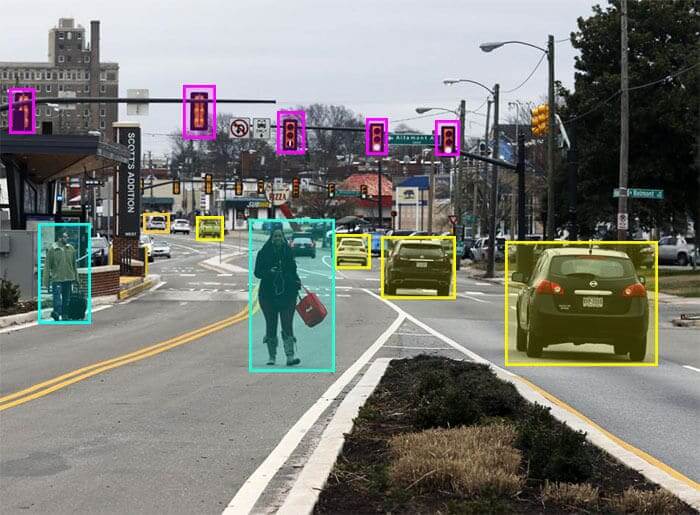
Figure: Image with multiple bounding box annotations per image </p> </div> <p>Another example is mask annotations, where each image is accompanied by a binary mask. The mask indicates what pixels in the image correspond to an object. The dataset can include the following information:</p> <div class="language-plaintext highlighter-rouge"><div class="highlight"><pre class="highlight"><code>	Image1: class a, binary mask
	Image2: class b, binary mask
	Image3: class a, binary mask
</code></pre></div></div> <div style="text-align: center; margin: 20px 0;"> <img src="https://cdn.prod.website-files.com/614c82ed388d53640613982e/63f498f8d4fe7da3b3a60cc2_semantic%20segmentation%20vs%20instance%20segmentation.jpg" style="width: 100%; max-width: 400px; height: auto; border-radius: 8px;"/> <p style="font-style: italic; font-size: 0.9em; margin-top: 10px; color: #666;"> Figure: Image with multiple mask annotations per image (source: [Link](https://www.superannotate.com/blog/guide-to-semantic-segmentation)) </p> </div> <p>Object detection is a popular example of a problem that requires bounding box annotations. Given an image, all the objects of interest are labeled with a bounding box. The task of object detection is to take an image as input and to identify and localize objects in the image. Examples:</p> <ul> <li>COCO: <a href="https://cocodataset.org/#home">Link</a></li> <li>PASCAL VOC: <a href="https://www.kaggle.com/datasets/gopalbhattrai/pascal-voc-2012-dataset">Link</a></li> </ul> <p>Segmentation is an example where mask annotations are needed. Some segmentation problems are well defined; examples include background segmentation, object segmentation, scene segmentation, etc. Example</p> <ul> <li>COCO (also provides masks for objects): <a href="https://cocodataset.org/#home">Link</a></li> </ul> <p>Fine-grained annotations, in the context of videos, can simply include bounding box annotations or mask annotations for each image in the video.</p> <p>Other types of annotation may include annotations for temporal video segmentation, where a video is divided into distinct scenes. Or labels for anomaly detection that can be both fine-grained or coarse-grained, etc. Other examples of video datasets:</p> <ul> <li>UCF-crime: <a href="https://www.kaggle.com/datasets/minhajuddinmeraj/anomalydetectiondatasetucf">Link</a></li> </ul> <p>Accurate fine-grained annotations are of great value for many problems, but are also extremely time-consuming and tedious to generate.</p> <h4 id="audio-data">Audio Data</h4> <p>Audio data, like visual data, can be annotated to train machine learning models. The annotations range from coarse, whole-audio labels to fine-grained, time-specific annotations. The choice of annotation type depends on the specific problem being addressed, such as music genre classification, speech recognition, or sound event detection.</p> <h5 id="coarse-annotations-1">Coarse Annotations</h5> <p>Coarse annotations for audio data typically apply to the entire audio clip and don’t provide temporal information. This is similar to how image classification provides a single label for a whole image.</p> <p>Audio classification is a broad category where the goal is to assign a single label to an entire audio clip. This can include: Music Genre Classification, where the objective is to identify the genre of a song (e.g., rock, classical, jazz). The dataset for this problem consists of audio files and one corresponding genre label per file. Examples:</p> <ul> <li>GTZAN: <a href="https://www.kaggle.com/datasets/andradaolteanu/gtzan-dataset-music-genre-classification">Link</a></li> <li>Million Song Dataset: <a href="http://millionsongdataset.com/">Link</a></li> </ul> <p>Speech/Speaker Identification determines who is speaking or if the audio contains speech. The label could be the speaker’s identity or simply “speech” or “non-speech.” Examples:</p> <ul> <li>LibriSpeech: <a href="https://www.openslr.org/12">Link</a></li> <li>VoxCeleb: <a href="https://www.robots.ox.ac.uk/~vgg/data/voxceleb/">Link</a></li> </ul> <h5 id="fine-grained-annotations-1">Fine-Grained Annotations</h5> <p>Fine-grained annotations for audio data include temporal information, pinpointing where specific sounds or events occur within an audio file. This is crucial for tasks that require precise localization. This type of annotation provides timestamps for specific events or segments within an audio file. An audio file of a busy street might have annotations like:</p> <div class="language-plaintext highlighter-rouge"><div class="highlight"><pre class="highlight"><code>0.5s - 2.0s: 'car horn'
3.2s - 4.5s: 'siren'
6.0s - 7.5s: 'dog bark'
</code></pre></div></div> <p>Sound Event Detection (SED) is a good example of a problem that requires fine-grained annotations. The goal is to identify and localize sounds in an audio clip by providing start and end times for each sound event. This is similar to object detection in images. Examples:</p> <ul> <li>DCASE Datasets: <a href="https://dcase.community/">Link</a></li> <li>AudioSet: <a href="https://research.google.com/audioset/">Link</a></li> </ul> <p>Like fine-grained visual annotations, creating high-quality fine-grained audio annotations is extremely time-consuming and labor-intensive. It requires human annotators to listen carefully and mark the precise start and end points of events, making it a valuable but costly part of dataset creation.</p> <h4 id="textual-data">Textual Data</h4> <p>Just like images, video, and audio, textual data requires annotation to become useful for training AI models, especially in the field of Natural Language Processing (NLP). The process, often called text annotation or data labeling, involves tagging or labeling text to give it structure and meaning that a machine can understand.</p> <h5 id="coarse-annotations-2">Coarse Annotations</h5> <p>Similar to image or audio classification, coarse annotations for text involve assigning a single label to an entire document, paragraph, or sentence. This type of annotation is used for problems where the overall meaning or characteristic of the text is the primary focus. Many problems fall under the broad area of text classification. Sentiment Analysis: This is a very common example. An entire block of text, like a product review or a social media post, is labeled as “positive,” “negative,” “neutral,” or even with a more specific emotion like “joy,” “anger,” or “sadness.” Example: Social Media Sentiment: <a href="https://www.kaggle.com/datasets/kashishparmar02/social-media-sentiments-analysis-dataset">Link</a> Amazon Reviews: <a href="https://www.kaggle.com/datasets/bittlingmayer/amazonreviews">Link</a></p> <h5 id="fine-grained-annotations-2">Fine-Grained Annotations</h5> <p>Fine-grained annotations for text are more detailed, providing information about specific words, phrases, or relationships within the text. This is analogous to bounding boxes or masks in visual data. Named Entity Recognition (NER): This is one of the most fundamental fine-grained text annotation tasks. It involves identifying and labeling proper nouns or other specific entities. Example annotation: In the sentence “Steve Jobs co-founded Apple in Cupertino,” the annotations would be:</p> <div class="language-plaintext highlighter-rouge"><div class="highlight"><pre class="highlight"><code>"Steve Jobs": PERSON
"Apple": ORGANIZATION
"Cupertino": LOCATION
</code></pre></div></div> <p>Example:</p> <ul> <li>NER: <a href="https://www.kaggle.com/datasets/naseralqaydeh/named-entity-recognition-ner-corpus">Link</a></li> </ul> <h4 id="influential-datasets">Influential Datasets</h4> <p>Not all datasets are the same; some have such a deep influence on today’s advancements that the majority of the AI/ML models that one may find in multimedia research are usually pretrained on these datasets. Let’s consider the following:</p> <h5 id="visual-understanding-problems">Visual understanding problems</h5> <p>Imagenet is a large-scale dataset with 14 million images spanning across 20k categories. The dataset initially contained coarse labels, one category name for each image, and was later expanded to have fine-grained bounding box annotations. It was accomplished by crowd-sourcing the annotation work using Amazon Mechanical Turk, and it took nearly 2 years and around 50K participants to have the first version of the dataset.</p> <p>The majority of the visual recognition tasks today, be it for video or images, use neural nets trained on Imagenet as a backbone to extract features to use them in downstream tasks.</p> <p>COCO from Microsoft is also a cornerstone dataset for object detection, segmentation, and image captioning. It contains over 330,000 images with detailed annotations for 80 object categories. Also annotated using crowdsourcing.</p> <h5 id="audio-understanding-problems">Audio understanding problems</h5> <p><em>AudioSet</em> is a massive dataset of over 5 million YouTube videos, each annotated with labels from an ontology of 527 sound events. It’s the most common dataset used for pre-training models for tasks like sound event detection and audio classification.</p> <p><em>LibriSpeech</em> is the definitive dataset for speech recognition. It’s a corpus of nearly 1,000 hours of English speech from audiobooks, all with corresponding text transcripts. Models like Wav2Vec and its successors, which have revolutionized speech recognition, are frequently pre-trained on this and similar large, unlabeled speech corpora to learn general speech features before being fine-tuned for specific tasks.</p> <p>While these are large-scale datasets, they are not annotated via crowdsourcing. AudioSet is manually labeled by human annotators, and LibriSpeech is derived from existing audiobooks.</p> <h5 id="textual-analysis-problems">Textual analysis problems</h5> <p>BooksCorpus (800 million words) and the English Wikipedia (2.5 billion words) are two large-scale datasets. BERT (Bidirectional Encoder Representations from Transformers) by Google was a breakthrough in NLP. Fine-tuning a pre-trained BERT model has become a standard approach for a wide range of tasks, from question answering to sentiment analysis.</p> <p>The Common Crawl dataset contains petabytes of web data and a variety of books, articles, and other internet texts. OpenAI’s GPT series is trained on these datasets and is often used as a starting point for developing new language models.</p> <p>Textual datasets like these are annotations in themselves, or do not need annotations for tasks like training LLMs.</p> <h4 id="emerging-directions-of-research">Emerging directions of research</h4> <p>A few directions of research that may be of interest to us. Multimodal AI AI models that are trained on multiple modalities (text, audio, video) are becoming increasingly relevant. Research in these areas focuses.</p> <ul> <li>Methods to extract common features from two or more modalities with the same semantic meaning.</li> <li>Methods to fuse features from various modalities.</li> <li>Cross-attention models that dynamically understand the importance of features across modalities. etc.</li> </ul> <h5 id="example-datasets-and-applications">Example datasets and applications</h5> <p>COCO’s VQA dataset is a text and image modal dataset for AI. These datasets allow for solving Vision-and-Language (V&amp;L) tasks like Visual Question Answering (VQA), multimedia data retrieval, image captioning, etc.</p> <p>YouTube-8M and MuSe (Multimodal Sentiment Analysis), which combines video and audio to analyze emotions Human-Centric AI Datasets are becoming more focused on capturing complex human behavior, interactions, and safety-critical scenarios. This is particularly relevant for applications in social robotics, healthcare, and safety systems.</p> <p>Example datasets and applications Egocentric Video Datasets (e.g., Ego4D) are collected from a first-person perspective (e.g., using a camera on a headset). They are crucial for understanding human-object interaction and for training models that can assist with daily tasks</p> <h4 id="some-insights">Some insights.</h4> <ul> <li>The most influential datasets are generally large, containing hundreds of thousands to millions of samples, and often rely on human annotators for fine-grained labels in image and audio modalities. Historically, these influential datasets have been made publicly available, fostering widespread research and innovation.</li> <li>However, it’s crucial to note that domain-specific, application-specific proprietary datasets can hold significant commercial value. The entities interested in these datasets are typically found in the private, commercial, retail, and public sectors, as they are tailored for specific business problems rather than general academic research.</li> </ul>]]></content><author><name></name></author><category term="datasets"/><category term="datasets"/><summary type="html"><![CDATA[Some insights on datasets!!]]></summary></entry><entry><title type="html">Imagenet-16</title><link href="https://pmantini.github.io/profile/blog/2026/imagenet-16/" rel="alternate" type="text/html" title="Imagenet-16"/><published>2026-02-03T14:24:00+00:00</published><updated>2026-02-03T14:24:00+00:00</updated><id>https://pmantini.github.io/profile/blog/2026/imagenet-16</id><content type="html" xml:base="https://pmantini.github.io/profile/blog/2026/imagenet-16/"><![CDATA[<ul id="markdown-toc"> <li><a href="#imagenet-16-a-lightweight-benchmark-for-few-shot-learning" id="markdown-toc-imagenet-16-a-lightweight-benchmark-for-few-shot-learning">ImageNet-16: A Lightweight Benchmark for Few-Shot Learning</a> <ul> <li><a href="#what-is-few-shot-classification" id="markdown-toc-what-is-few-shot-classification">What is Few-Shot Classification?</a></li> <li><a href="#the-standard-protocol-1-2-4-8-and-16-shots" id="markdown-toc-the-standard-protocol-1-2-4-8-and-16-shots">The Standard Protocol: 1, 2, 4, 8, and 16 Shots</a></li> <li><a href="#the-imagenet-hurdle" id="markdown-toc-the-imagenet-hurdle">The ImageNet Hurdle</a></li> <li><a href="#introducing-imagenet-16" id="markdown-toc-introducing-imagenet-16">Introducing ImageNet-16</a></li> <li><a href="#license-and-integrity" id="markdown-toc-license-and-integrity">License and Integrity</a></li> <li><a href="#why-scale-matters-for-multimodal-alignment" id="markdown-toc-why-scale-matters-for-multimodal-alignment">Why Scale Matters for Multimodal Alignment</a></li> <li><a href="#citation" id="markdown-toc-citation">Citation</a></li> </ul> </li> </ul> <div style="text-align: center; margin: 30px 0;"> <a href="https://drive.google.com/file/d/11ekx77JyDoY2-KluCNrgLwqULWXtT_bV/view?usp=sharing" class="btn btn-outline-primary btn-lg" target="_blank" rel="noopener noreferrer"> <i class="fas fa-download"></i> Download ImageNet-16 (1.8 GB) </a> </div> <h2 id="imagenet-16-a-lightweight-benchmark-for-few-shot-learning">ImageNet-16: A Lightweight Benchmark for Few-Shot Learning</h2> <h4 id="what-is-few-shot-classification">What is Few-Shot Classification?</h4> <p><strong>Image classification</strong> is a fundamental problem in computer vision, where the objective is to categorize images into predefined semantic classes. In standard deep learning, we typically assume that “data is cheap”. To teach a model to recognize a “Golden Retriever,” we feed it thousands of labeled examples. However, in the real world, data is often expensive, rare, or private.</p> <p><strong>Few-shot classification</strong> is a more restrictive formulation where only a limited number of labeled samples are available for training—a constraint that is far more representative of real-world scenarios.</p> <h4 id="the-standard-protocol-1-2-4-8-and-16-shots">The Standard Protocol: 1, 2, 4, 8, and 16 Shots</h4> <p>To measure how well an algorithm learns from limited data, the community has settled on a standardized “shot” protocol.</p> <ul> <li> <p>k-shot: This refers to the number of training samples available per class.</p> </li> <li> <p>The Benchmarking Ladder: Most papers, including our recent work on <a href="https://arxiv.org/pdf/2603.08942">BiCLIP</a>, evaluate models across 1, 2, 4, 8, and 16 shots.</p> </li> </ul> <p>By testing across this spectrum, we can see the “learning curve” of an architecture. Does the model accuracy improve from 1 shot to 16 shot? This delta tells us how efficiently the model utilizes every new piece of information.</p> <h4 id="the-imagenet-hurdle">The ImageNet Hurdle</h4> <p>ImageNet (specifically ImageNet-1K) remains the “Gold Standard” for internalizing visual concepts. However, it presents a massive logistical hurdle for many:</p> <ul> <li> <p>Size: The full dataset is ~150GB.</p> </li> <li> <p>Time: Downloading and extracting it can take hours, and training even a simple linear probe on the full set requires significant GPU memory and time.</p> </li> <li> <p>Redundancy: For few-shot research, you don’t actually need 1,300 images per class if you are only ever going to use 16 for training.</p> </li> </ul> <p>Most researchers end up writing their own scripts to “subsample” ImageNet, but these scripts vary, leading to slight inconsistencies in which specific images are used for the 16-shot sets.</p> <h4 id="introducing-imagenet-16">Introducing ImageNet-16</h4> <p>ImageNet-16 addresses this issue.</p> <p><strong>What is it?</strong></p> <p>It is a curated subset of the original ImageNet-1K. It contains exactly 16 samples per class for all 1,000 classes.</p> <p>Total Images: 16,000 (compared to 1.2 million).</p> <p>Total Size: Under 2GB (compared to 150GB).</p> <p>Evaluation: The evaluation is performed on the original ImageNet validation set. This ensures that your few-shot results are directly comparable to the state-of-the-art results reported in major CVPR/ICCV papers.</p> <h4 id="license-and-integrity">License and Integrity</h4> <p>It is important to note that ImageNet-16 is a derivative work.</p> <p>License: This subset is distributed under the same non-commercial research license dictated by the original ImageNet (Stanford/Princeton).</p> <p>Fixed Seeds: The 16 samples were selected using a fixed random seed to ensure that anyone using this dataset is training on the exact same “anchors.”</p> <h4 id="why-scale-matters-for-multimodal-alignment">Why Scale Matters for Multimodal Alignment</h4> <p>This dataset was born out of my work on <a href="https://arxiv.org/pdf/2603.08942">BiCLIP</a>. In that paper, we hypothesized that the gap between different domains (like satellite imagery vs. generic objects) can be bridged using a geometric transformation.</p> <p>To recover this transformation, we need “anchors”—the few-shot samples. By using a lightweight dataset like ImageNet-16, we can iterate on these alignment algorithms in minutes rather than days, proving that you don’t need “Big Data” to achieve “Big Results” in cross-modal alignment.</p> <div style="background: #f8f9fa; border-left: 5px solid #007bff; padding: 20px; border-radius: 5px; margin: 25px 0;"> <h4 style="margin-top: 0;"><i class="fas fa-database"></i> Access the Dataset</h4> <p>The 16-shot ImageNet subset is hosted externally for easy access:</p> <ul> <li><strong>Dataset:</strong> <a href="https://drive.google.com/file/d/11ekx77JyDoY2-KluCNrgLwqULWXtT_bV/view?usp=sharing">Download ImageNet-16 (.zip)</a></li> <li><strong>Labels:</strong> <a href="https://github.com/HoldenCaulfieldRye/caffe/blob/master/data/ilsvrc12/synset_words.txt">synset_words.txt</a></li> <li><strong>Paper:</strong> <a href="https://arxiv.org/abs/2603.08942">BiCLIP on arXiv</a></li> <li><strong>Imagenet-1K:</strong> <a href="https://www.image-net.org/about.php">Official Imagenet website</a></li> </ul> <p style="font-size: 0.85em; color: #666; margin-bottom: 0;"> <em>Note: Please ensure you comply with the original ImageNet Research License.</em> </p> </div> <h4 id="citation">Citation</h4> <p>Cite the original Imagenet dataset if using this dataset</p> <div class="language-plaintext highlighter-rouge"><div class="highlight"><pre class="highlight"><code>@inproceedings{deng2009imagenet,
  title={ImageNet: A Large-Scale Hierarchical Image Database},
  author={Deng, Jia and Dong, Wei and Socher, Richard and Li, Li-Jia and Li, Kai and Fei-Fei, Li},
  booktitle={IEEE Conference on Computer Vision and Pattern Recognition},
  pages={248--255},
  year={2009}
}
</code></pre></div></div> <p>Additionally, if this specific 16-shot sampling was useful for your work, please consider citing the BiCLIP paper where this subset was first introduced:</p> <div class="language-plaintext highlighter-rouge"><div class="highlight"><pre class="highlight"><code>@misc{mantini2026biclipdomaincanonicalizationstructured,
      title={BiCLIP: Domain Canonicalization via Structured Geometric Transformation}, 
      author={Pranav Mantini and Shishir K. Shah},
      year={2026},
      eprint={2603.08942},
      archivePrefix={arXiv},
      primaryClass={cs.CV},
      url={https://arxiv.org/abs/2603.08942}, 
}
</code></pre></div></div>]]></content><author><name></name></author><category term="datasets"/><category term="datasets"/><summary type="html"><![CDATA[16-Shot Imagenet Dataset]]></summary></entry><entry><title type="html">ADOC | Pranav Mantini</title><link href="https://pmantini.github.io/profile/blog/2026/adoc-pranav-mantini/" rel="alternate" type="text/html" title="ADOC | Pranav Mantini"/><published>2026-01-08T00:00:00+00:00</published><updated>2026-01-08T00:00:00+00:00</updated><id>https://pmantini.github.io/profile/blog/2026/adoc--pranav-mantini</id><content type="html" xml:base="https://pmantini.github.io/profile/blog/2026/adoc-pranav-mantini/"><![CDATA[<p>A Day on Campus Dataset. An Anomaly Detection Dataset for Events in a Single Camera.Visual examples from the ADOC dataset showing diverse events under varying conditions.Golf Cart on WalkwayPerson on GrassPerson on SkateboardHaving a ConversationRiding Bike (Day)Person with UmbrellaMobility ScooterRiding Bike (Night)The ADOC dataset is a foundational resource for anomaly detection in single-camera surveillance. We acquired 24 continuous hours of 1080p, H.264 video from a live university campus. The data encapsulates extreme variations in illumination, background clutter, and crowd density.We define anomalies as statistically “rare” events (low-frequency occurrences). Our data is meticulously annotated with 875 events, including high-frequency actions and specific rare activities like “golf cart on walkway” or “person with a mobility scooter.”</p>]]></content><author><name></name></author><category term="internal-posts"/><category term="datasets"/><summary type="html"><![CDATA[A Day on Campus Dataset. An Anomaly Detection Dataset for Events in a Single Camera.]]></summary></entry><entry><title type="html">UHCTD | Pranav Mantini</title><link href="https://pmantini.github.io/profile/blog/2026/uhctd-pranav-mantini/" rel="alternate" type="text/html" title="UHCTD | Pranav Mantini"/><published>2026-01-08T00:00:00+00:00</published><updated>2026-01-08T00:00:00+00:00</updated><id>https://pmantini.github.io/profile/blog/2026/uhctd--pranav-mantini</id><content type="html" xml:base="https://pmantini.github.io/profile/blog/2026/uhctd-pranav-mantini/"><![CDATA[<p>Camera Tampering Dataset. A Comprehensive Dataset for Synthetic Camera Tampering Detection.The University of Houston Camera Tampering Dataset (UHCTD) is a large-scale resource designed to train and evaluate algorithms for detecting unauthorized or accidental changes in surveillance views. Tampering—whether caused by natural phenomena like sunlight reflection and fog, or malicious human intent like spray painting and lens blocking—compromises the integrity of public safety systems.UHCTD features over 26GB of data captured from two high-resolution outdoor cameras (2048x1536 and 1280x960). We utilized advanced image processing techniques to synthesize three primary categories of tampering into real-world surveillance footage:The project includes a comprehensive evaluation of standard deep learning architectures for tampering detection, including:</p>]]></content><author><name></name></author><category term="internal-posts"/><category term="datasets"/><summary type="html"><![CDATA[Camera Tampering Dataset. A Comprehensive Dataset for Synthetic Camera Tampering Detection.]]></summary></entry></feed>